3 The Cantor set
This
is part of a longer thesis advancing a refutation of strong AI. To download the thesis visit: -
For an introduction to the work as a
whole visit: -
Introduction
to Poincare’s thesis by Peter Fekete
The Cantor set
occupies a unique mid-position between our two conceptions of infinite analytic
logic. On the one hand it is the maximal
structure of the analytic logic of ![]() and is the
Boolean lattice over which that logic is built; on the other hand it is a
necessary subspace of the continuum and therefore a fundamental sub-structure
over which the analytic logic of the continuum is constructed.
and is the
Boolean lattice over which that logic is built; on the other hand it is a
necessary subspace of the continuum and therefore a fundamental sub-structure
over which the analytic logic of the continuum is constructed.
3.1 (+) Aside, the analytic logic of the continuum
There appears to be
an analytic logic of the continuum that is not expressed, for instance, in the
formal analytic logic of the predicate calculus. Analytic logic is based on the fundamental
idea of containment. The predicate logic
interprets this principle by means of an analysis of the continuum into a
discrete skeleton of ![]() parts over which a
lattice is constructed and on top of that analytic logic is built. But there are analytic relations in the
continuum not encompassed or seen by this logic.
parts over which a
lattice is constructed and on top of that analytic logic is built. But there are analytic relations in the
continuum not encompassed or seen by this logic.
3.2 Iterative
definition of the Cantor set
Because of this
construction the Cantor set is also known as the Cantor ternary set, and
also designated ![]() , denoting a Smith-Voltarra-Cantor
set.[1] Let
, denoting a Smith-Voltarra-Cantor
set.[1] Let
![]() . Remove from this the
middle open third, that is the interval
. Remove from this the
middle open third, that is the interval ![]() , to obtain
, to obtain ![]() . Remove from each
part of this its middle open third, to obtain
. Remove from each
part of this its middle open third, to obtain ![]() . Iterate this process
to obtain a sequence of closed sets
. Iterate this process
to obtain a sequence of closed sets ![]() each of which contains
all of its successors. Define the Cantor
set by
each of which contains
all of its successors. Define the Cantor
set by ![]() . This is a closed
set. F contains all the points
that remain after all the open intervals in the sequence
. This is a closed
set. F contains all the points
that remain after all the open intervals in the sequence ![]() have been
removed. It therefore contains all the end-points
of these intervals,
have been
removed. It therefore contains all the end-points
of these intervals, ![]() . It can be shown
that the Cantor set “contains a multitude of points
other than the above end-points, for the set of these end-points is clearly
countable, while the cardinal number of F itself is c, the
cardinal number of the continuum.” (Simmons [1963] p. 67.)
. It can be shown
that the Cantor set “contains a multitude of points
other than the above end-points, for the set of these end-points is clearly
countable, while the cardinal number of F itself is c, the
cardinal number of the continuum.” (Simmons [1963] p. 67.)
3.3 The puzzle
of the Cantor set
This remark by Simmons is indicative of a significant
puzzle when we consider the Cantor set.
The members of this set are all enclosed within intervals of zero
measure, whose endpoints are a set of cardinality ![]() ; nonetheless the cardinality of the members of the Cantor
set is
; nonetheless the cardinality of the members of the Cantor
set is ![]() . How is it possible
for
. How is it possible
for ![]() points to be enclosed in
points to be enclosed in
![]() intervals?
intervals?
3.4 Result, ternary
representation of an element of the Cantor set
The elements of the Cantor
ternary set are those numbers that can be written in base 3 without using the
digit 1.
Proof
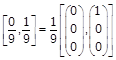
Consider the base 3 expansion
of numbers between 0 and 1. This
expansion uses only the digits 0, 1 and 2.
Example
![]()
Call such a base 3 representation of a
fraction a ternary fraction.
Observe also that any finite ternary fraction can be written as infinite
ternary fraction with repeating 2s. For
example, the ternary fractions
![]()
Now consider the construction of the
Cantor set.
Iterate Remove Removed as an infinite What is
left as an infinite ternary fraction* ternary fraction
1 ![]()
![]()
![]()
2 ![]()
![]()
Note
* 0.1 is not removed. That is why I have put it in brackets. What is removed is the open interval from 0.1
to 0.111... etc.
We see that at every iteration the ternary fractions that we remove are
those that as infinite (but not finite) ternary fractions contain a 1,
and those that are left are those that as finite or infinite ternary fractions
use only the digits 0 and 2. After a countably infinite number of iterations we have as the
elements of the Cantor set only those numbers that can be written in base 3 as
infinite ternary fractions without using the digit 1.
3.5 Example
The fraction ![]() is contained in the
Cantor set and yet is not an end-point of any closed interval in it. To show this, observe that: -
is contained in the
Cantor set and yet is not an end-point of any closed interval in it. To show this, observe that: -
![]() .[2]
.[2]
By examination of the
iterative process above we see that the end-points of any closed interval in
the Cantor set terminate in strings of the form: -
![]()
The first case only
occurs in the case of ![]() . Thus any infinite ternary fraction that can
be written with 0 and 2s that recur in any other pattern is an element
contained in the Cantor set, but not identical to an end point of any
closed interval in the Cantor set. This
example illustrates the puzzle of the Cantor set. [3.3 above]
. Thus any infinite ternary fraction that can
be written with 0 and 2s that recur in any other pattern is an element
contained in the Cantor set, but not identical to an end point of any
closed interval in the Cantor set. This
example illustrates the puzzle of the Cantor set. [3.3 above]
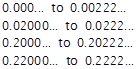
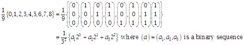
3.6 Result,
canonical representation of the Cantor set, the
Devil’s staircase
Let x be an element in the
Cantor set. Take the base 3 expansion of
x. Convert each 2 in that
expansion to a 1 and then read the number as a base 2 number. This
function is said to be the Devil’s Staircase, also called the Lebesgue singular function and maps all of C onto ![]() .
.
Example
![]()
Thus the canonical representation of
the Cantor set is the set ![]() . The set
. The set ![]() is equinumerous
with the Cantor set. There are c
many points in the Cantor set.
is equinumerous
with the Cantor set. There are c
many points in the Cantor set.
Proof
The Cantor construction starts with an
interval ![]() with end points
with end points ![]() . At the first
iteration this is subdivided into closed and open sets with end points:
. At the first
iteration this is subdivided into closed and open sets with end points:
![]() .
.
At the second iteration this is further
subdivided into closed and open intervals with end points: -
And so on. So any such binary sequence may be mapped to
a real number by: -
![]() and
in the limit,
and
in the limit, ![]() .
.
This displays the isomorphism of the
set of reals to the end-points of the Cantor set, and any SVC set
[Defined, footnote 2 above]. However, in
the Cantor set certain intervals are designated as in the set and
certain intervals are designated as not in the set. When n is finite, each interval that
is in the set is designated by two finite binary sequences. For example, the first interval at the 2nd
iteration is: -
But in the limit as ![]() the two adjacent
end-point sequences converge on a unique single real number with a single
binary representation. Each of these
points is in he Cantor
set. So the mapping is a mapping
of the Cantor set onto the reals. Each
interval in the Cantor set is identified with a unique real number.
the two adjacent
end-point sequences converge on a unique single real number with a single
binary representation. Each of these
points is in he Cantor
set. So the mapping is a mapping
of the Cantor set onto the reals. Each
interval in the Cantor set is identified with a unique real number.
3.7 The puzzle
The
Cantor set contains continuum many, c, additional points that are not its
end points. [See Chap. 2 / 2.7.10.] We have seen that that ![]() is one such
point. It may be noted, that whilst the
Cantor set contains c many points, the length of the segment removed is
equal to 1, since
is one such
point. It may be noted, that whilst the
Cantor set contains c many points, the length of the segment removed is
equal to 1, since ![]() . Conversely, when we
remove the Cantor set from the interval
. Conversely, when we
remove the Cantor set from the interval ![]() we remove a set with c
many points but leave an interval of length
we remove a set with c
many points but leave an interval of length ![]() behind.
behind.
Diagram of the
Devil’s staircase
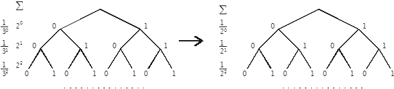
The
end-points of the Cantor set are given on the left, and the elements of ![]() are given on the
right. It is said that there are
are given on the
right. It is said that there are ![]() points in the left
tree and
points in the left
tree and ![]() in the right
tree. This appears to be a paradox. That there are
in the right
tree. This appears to be a paradox. That there are ![]() points on the left is
argued that there are countably infinite branches,
each designating an end-point. That
there are
points on the left is
argued that there are countably infinite branches,
each designating an end-point. That
there are ![]() points on the right is
argued by the claim that it is the power set of
points on the right is
argued by the claim that it is the power set of ![]() .
.
3.8 Resolution of this
paradox
The resolution is
that the number and length of the branches on the left is not ![]() but
but ![]() ; on the right it is
; on the right it is ![]() . So there are many
more points on the right than on the left. This gives an injection of the set of
end-points with the set
. So there are many
more points on the right than on the left. This gives an injection of the set of
end-points with the set ![]() . The end points are
generated by
. The end points are
generated by ![]() iterations and the
points themselves are generated by
iterations and the
points themselves are generated by ![]() iterations. The result of both limiting processes is the
same – to produce closed sets of zero measure.
iterations. The result of both limiting processes is the
same – to produce closed sets of zero measure.
3.9
(+) Theorem, ![]()
We have
just demonstrated ![]() .
.
Proof
By contradiction. Assume
![]() , then the number of iterations in the construction of the
end-points of the Cantor set is equal to the number of iterations in the
construction of the Cantor set itself.
This implies
, then the number of iterations in the construction of the
end-points of the Cantor set is equal to the number of iterations in the
construction of the Cantor set itself.
This implies ![]() , whence
, whence ![]() .
.
What this illustrates
is that the distinction between ![]() and
and ![]() is essential to mathematics and is everywhere implicit. It shows up, for instance, in the distinction
between
is essential to mathematics and is everywhere implicit. It shows up, for instance, in the distinction
between ![]() and
and ![]() , the latter marking the disguised presence of
, the latter marking the disguised presence of ![]() . The Cantor set is
defined by an actual, completed construction, and is the product:
. The Cantor set is
defined by an actual, completed construction, and is the product: ![]() ; the end-points of the Cantor set in the ternary
construction are defined by a recursive (inductive) procedure over the
unbounded, potentially infinite collection
; the end-points of the Cantor set in the ternary
construction are defined by a recursive (inductive) procedure over the
unbounded, potentially infinite collection ![]() , and hence may be written
, and hence may be written ![]() which makes
the set of end
points into the sub-direct product of an indeterminate but countably
infinite number of copies of
which makes
the set of end
points into the sub-direct product of an indeterminate but countably
infinite number of copies of ![]() . Equating
the two leads to paradox. This
solution is also reflected in set theory in the distinction between ordinal and
cardinal exponentiation
. Equating
the two leads to paradox. This
solution is also reflected in set theory in the distinction between ordinal and
cardinal exponentiation
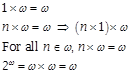
3.10 Examples of
ordinal multiplication
Ordinal mulitplication
is based on the concept of order types.
1. ![]() (ordinal
multiplication) .
(ordinal
multiplication) .
![]() is
ordered by
is
ordered by ![]() which is
order-isomorphic to
which is
order-isomorphic to ![]() .
.
2, ![]() (ordinal
multiplication).
(ordinal
multiplication).
![]() is
ordered by
is
ordered by ![]() which is
order-isomorphic to
which is
order-isomorphic to ![]() .
.
3.11 Ordinal
exponentiation is not the same as cardinal exponentiation
Cardinal arithmetic is concerned with
the operations of union, Cartesian product and ![]() , the class of all functions from Y into X. Therefore, ordinal exponentiation
, the class of all functions from Y into X. Therefore, ordinal exponentiation
![]() , in spite of the ambiguous notation, has nothing to do with
the operation of forming
, in spite of the ambiguous notation, has nothing to do with
the operation of forming ![]() . Thus, for example:
. Thus, for example:
Ordinal exponentiation ![]()
Cardinal exponentiation ![]()
Regarding
![]() (ordinal
exponentiation). This proceeds by
induction: -
(ordinal
exponentiation). This proceeds by
induction: -
In set theory ordinal
exponentiation is extended by definition to transfinite ordinals. The ordinal exponent ![]() (note, not bold type)
should perhaps be better written
(note, not bold type)
should perhaps be better written ![]() . It is a potentially
infinite collection equinumerous to
. It is a potentially
infinite collection equinumerous to
![]() .
.
3.12 Cantor space
There is a good deal more that can be said about the Cantor set and the
Cantor space with which it is synonymous.
This material is extraneous to our purpose here – which is to examine
the validity of Poincaré’s thesis. I note in passing, Brower’s theorem: A topological space is
a Cantor space iff it is non-empty,
perfect, compact, totally
disconnected and metrizable. Explication of this result takes us too far
from our subject, which requires only examination of the Cantor set as the
essential model of formal, analytic logic, and provides us with a vehicle to
demonstrate the validity of the thesis that complete induction is not a
principle of analytic reasoning.
This
is part of a longer thesis advancing a refutation of strong AI. To download the thesis visit: -
For an introduction to the work as a
whole visit: -
Introduction
to Poincare’s thesis by Peter Fekete